Quantum finite automata

In quantum computing, quantum finite automata or QFA are a quantum analog of probabilistic automata. They are related to quantum computers in a similar fashion as finite automata are related to Turing machines. Several types of automata may be defined, including measure-once and measure-many automata. Quantum finite automata can also be understood as the quantization of subshifts of finite type, or as a quantization of Markov chains. QFA's are, in turn, special cases of geometric finite automata or topological finite automata.

The automata work by accepting a finite-length string $\sigma=(\sigma_0,\sigma_1,\cdots,\sigma_k)$ of letters $\sigma_i$ from a finite alphabet $\Sigma\ni\sigma_i$ , and assigning to each such string a probability $\operatorname{Pr}(\sigma)$ indicating the probability of the automaton being in an accept state; that is, indicating whether the automaton accepted or rejected the string.

1 Measure-once automata
2 Example
3 Measure-many automata
4 Geometric generalizations
5 See also
6 References

Measure-once automata

Measure-once automata were introduced by Moore and Crutchfield^[1]. They may be defined formally as follows.

As with an ordinary finite automaton, the quantum automaton is considered to have $N$ possible internal states, represented in this case by an $N$ -state qubit $|\psi\rangle$ . More precisely, the $N$ -state qubit $|\psi\rangle\in \mathbb {C}P^N$ is an element of $N$ -dimensional complex projective space, carrying an inner product $\Vert\cdot\Vert$ that is the Fubini-Study metric.

The state transitions, transition matrixes or de Bruijn graphs are represented by a collection of $N\times N$ unitary matrixes $U_\alpha$ , with one unitary matrix for each letter $\alpha\in\Sigma$ . That is, given an input letter $\alpha$ , the unitary matrix describes the transition of the automaton from its current state $|\psi\rangle$ to its next state $|\psi^\prime\rangle$ :

$|\psi^\prime\rangle = U_\alpha |\psi\rangle$

Thus, the triple $(\mathbb {C}P^N,\Sigma,\{U_\alpha\vert\alpha\in\Sigma\})$ form a quantum semiautomaton.

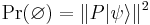
The accept state of the automaton is given by an $N\times N$ projection matrix $P$ , so that, given a $N$ -dimensional quantum state $|\psi\rangle$ , the probability of $|\psi\rangle$ being in the accept state is

$\langle\psi |P |\psi\rangle = \Vert P |\psi\rangle\Vert^2$

The probability of the state machine accepting a given finite input string $\sigma=(\sigma_0,\sigma_1,\cdots,\sigma_k)$ is given by

$\operatorname{Pr}(\sigma) = \Vert P U_{\sigma_k} \cdots U_{\sigma_1} U_{\sigma_0}|\psi\rangle\Vert^2$

Here, the vector $|\psi\rangle$ is understood to represent the initial state of the automaton, that is, the state the automaton was in before it stated accepting the string input. The empty string $\varnothing$ is understood to be just the unit matrix, so that

$\operatorname{Pr}(\varnothing)= \Vert P |\psi\rangle\Vert^2$

is just the probability of the initial state being an accepted state.

Because the left-action of $U_\alpha$ on $|\psi\rangle$ reverses the order of the letters in the string $\sigma$ , it is not uncommon for QFA's to be defined using a right action on the Hermitian transpose states, simply in order to keep the order of the letters the same.

A regular language is accepted with probability $p$ by a quantum finite automaton, if, for all sentences $\sigma$ in the language, (and a given, fixed initial state $|\psi\rangle$ ), one has $p<\operatorname{Pr}(\sigma)$ .

Example

Consider the classical deterministic finite automaton given by the state transition table

**State Transition Table**
Input State	1	0
S₁	S₁	S₂
S₂	S₂	S₁

State Diagram

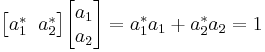
The quantum state is a vector, in bra-ket notation

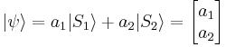
$|\psi\rangle=a_1 |S_1\rangle %2B a_2|S_2\rangle = \begin{bmatrix} a_1 \\ a_2 \end{bmatrix}$

with the complex numbers $a_1,a_2$ normalized so that

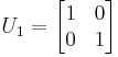
$\begin{bmatrix} a^*_1 \;\; a^*_2 \end{bmatrix} \begin{bmatrix} a_1 \\ a_2 \end{bmatrix} = a_1^*a_1 %2B a_2^*a_2 = 1$

The unitary transition matrices are

$U_0=\begin{bmatrix} 0 & 1 \\ 1 & 0 \end{bmatrix}$

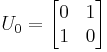
and

$U_1=\begin{bmatrix} 1 & 0 \\ 0 & 1 \end{bmatrix}$

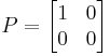
Taking $S_1$ to be the accept state, the projection matrix is

$P=\begin{bmatrix} 1 & 0 \\ 0 & 0 \end{bmatrix}$

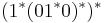
As should be readily apparent, if the initial state is the pure state $|S_1\rangle$ or $|S_2\rangle$ , then the result of running the machine will be exactly identical to the classical deterministic finite state machine. In particular, there is a language accepted by this automaton with probability one, for these initial states, and it is identical to the regular language for the classical DFA, and is given by the regular expression:

$(1^*(01^*0)^*)^* \,\!$

The non-classical behaviour occurs if both $a_1$ and $a_2$ are non-zero. More subtle behaviour occurs when the matrices $U_0$ and $U_1$ are not so simple; see, for example, the de Rham curve as an example of a quantum finite state machine acting on the set of all possible finite binary strings.

Measure-many automata

Measure-many automata were introduced by Kondacs and Watrous in 1997.^[2]. The general framework resembles that of the measure-once automaton, except that instead of there being one projection, at the end, there is a projection, or quantum measurement, performed after each letter is read. A formal definition follows.

The Hilbert space $\mathcal{H}_Q=\mathbb{C}P^N$ is decomposed into three orthogonal subspaces

$\mathcal{H}_Q=\mathcal{H}_\mbox{accept} \oplus \mathcal{H}_\mbox{reject} \oplus \mathcal{H}_\mbox{non-halting}$

In the literature, these orthogonal subspaces are usually formulated in terms of the set $Q$ of orthogonal basis vectors for the Hilbert space $\mathcal{H}_Q$ . This set of basis vectors is divided up into subsets $Q_\mbox{acc} \subset Q$ and $Q_\mbox{rej} \subset Q$ , such that

$\mathcal{H}_\mbox{accept}=\operatorname{span} \{|q\rangle�: |q\rangle \in Q_\mbox{acc} \}$

is the linear span of the basis vectors in the accept set. The reject space is defined analogously, and the remaining space is designated the non-halting subspace. There are three projection matrices, $P_\mbox{acc}$ , $P_\mbox{rej}$ and $P_\mbox{non}$ , each projecting to the respective subspace:

$P\mbox{acc}:\mathcal{H}_Q \to \mathcal{H}_\mbox{accept}$

and so on. The parsing of the input string proceeds as follows. Consider the automaton to be in a state $|\psi\rangle$ . After reading an input letter $\alpha$ , the automaton will be in the state

$|\psi^\prime\rangle =U_\alpha |\psi\rangle$

At this point, a measurement is performed on the state $|\psi^\prime\rangle$ , using the projection operators $P$ , at which time its wave-function collapses into one of the three subspaces $\mathcal{H}_\mbox{accept}$ or $\mathcal{H}_\mbox{reject}$ or $\mathcal{H}_\mbox{non-halting}$ . The probability of collapse is given by

$\operatorname{Pr}_\mbox{acc} (\sigma) = \Vert P_\mbox{acc} |\psi^\prime\rangle \Vert^2$

for the "accept" subspace, and analogously for the other two spaces.

If the wave function has collapsed to either the "accept" or "reject" subspaces, then further processing halts. Otherwise, processing continues, with the next letter read from the input, and applied to what must be an eigenstate of $P_\mbox{non}$ . Processing continues until the whole string is read, or the machine halts. Often, additional symbols $\kappa$ and $ are adjoined to the alphabet, to act as the left and right end-markers for the string.

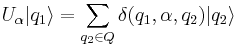
In the literature, the meaure-many automaton is often denoted by the tuple $(Q;\Sigma; \delta; q_0; Q_\mbox{acc}; Q_\mbox{rej})$ . Here, $Q$ , $\Sigma$ , $Q\mbox{acc}$ and $Q\mbox{rej}$ are as defined above. The initial state is denoted by $|\psi\rangle=|q_0\rangle$ . The unitary transformations are denoted by the map $\delta$ ,

$\delta:Q\times \Sigma \times Q \to \mathbb{C}$

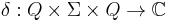
so that

$U_\alpha |q_1\rangle = \sum_{q_2\in Q} \delta (q_1, \alpha, q_2) |q_2\rangle$

Geometric generalizations

The above constructions indicate how the concept of a quantum finite automaton can be generalized to arbitrary topological spaces. For example, one may take some (N-dimensional) Riemann symmetric space to take the place of $\mathbb{C}P^N$ . In place of the unitary matrices, one uses the isometries of the Riemannian manifold, or, more generally, some set of open functions appropriate for the given topological space. The initial state may be taken to be a point in the space. The set of accept states can be taken to be some arbitrary subset of the topological space. One then says that a formal language is accepted by this topological automaton if the point, after iteration by the homeomorphisms, intersects the accept set. But, of course, this is nothing more than the standard definition of an M-automaton. The behaviour of topological automata is studied in the field of topological dynamics.

The quantum automaton differs from the topological automaton in that, instead of having a binary result (is the iterated point in, or not in, the final set?), one has a probability. The quantum probability is the (square of) the initial state projected onto some final state P; that is 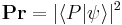$\bold{Pr} = \vert \langle P\vert \psi\rangle \vert^2$ . But this probability amplitude is just a very simple function of the distance between the point $\vert P\rangle$ and the point $\vert \psi\rangle$ in $\mathbb{C}P^N$ , under the distance metric given by the Fubini-Study metric. To recap, the quantum probability of a language being accepted can be interpreted as a metric, with the probability of accept being unity, if the metric distance between the initial and final states is zero, and otherwise the probability of accept is less than one, if the metric distance is non-zero. Thus, it follows that the quantum finite automaton is just a special case of a geometric automaton or a metric automaton, where $\mathbb{C}P^N$ is generalized to some metric space, and the probability measure is replaced by a simple function of the metric on that space.

References

^ C. Moore, J. Crutchfield, "Quantum automata and quantum grammars", Theoretical Computer Science, 237 (2000) pp 275-306.
^ Kondacs, A.; Watrous, J. (1997), "On the power of quantum finite state automata", Proceedings of the 38th Annual Symposium on Foundations of Computer Science, pp. 66–75

L. Accardi (2001), "Quantum stochastic processes", in Hazewinkel, Michiel, Encyclopedia of Mathematics, Springer, ISBN 978-1556080104, http://www.encyclopediaofmath.org/index.php?title=Q/q076330 (Provides an intro to quantum Markov chains.)
Alex Brodsky, Nicholas Pippenger, "Characterization of 1-way Quantum Finite Automata", SIAM Journal on Computing 31(2002) pp 1456-1478.
Vincent D. Blondel, Emmanual Jeandel, Pascal Koiran and Natacha Portier, "Decidable and Undecidable Problems about Quantum Automata", SIAM Journal on Computing 34 (2005) pp 1464-1473.

Quantum information science

General	Quantum computer • Qubit • Quantum information • Quantum programming • Timeline of quantum computing

Quantum communication	Quantum capacity • Quantum channel • Quantum cryptography (Quantum key distribution) • Quantum teleportation • Superdense coding • LOCC • Entanglement distillation

Quantum algorithms	Universal quantum simulator • Deutsch–Jozsa algorithm • Grover's search • quantum Fourier transform • Shor's factorization • Simon's Algorithm • Quantum phase estimation algorithm • Quantum annealing

Quantum complexity theory	Quantum Turing machine • BQP • QMA • PostBQP

Quantum computing models	Quantum circuit (Quantum gate) • One-way quantum computer (cluster state) • Adiabatic quantum computation • Topological quantum computer

Decoherence prevention	Quantum error correction • Stabilizer codes • Entanglement-Assisted Quantum Error Correction • Quantum convolutional codes

Physical implementations

Quantum optics	Cavity QED

Ultracold atoms	Trapped ion quantum computer • Optical lattice

Spin-based	Nuclear magnetic resonance QC • Kane QC • Loss–DiVincenzo QC • Nitrogen-vacancy center

Superconducting quantum computing	Charge qubit • Flux qubit • Phase qubit